Fix the model
We fixed Orbium’s update rule and one-kernel geometry, then searched for the three parameter values. Other update laws and kernel layouts are outside this comparison.
 SPECTER LABS
One mature frame of Orbium was enough for a search to recover its rule parameters close to the native values, once the rule family and the starting cells were known. Without that knowledge the problem is harder, and this report follows what a search needs to be given before it can find a rule that grows and keeps the body we actually want.
 Native rule
 Recovered rule
The desired body keeps its form through a continuous process of local change, so recovering it means finding dynamics that sustain the anatomy as well as an image that resembles it. We approached that problem with two requests. Supplying a complete body let us search for a rule that maintains it, and fixing a known rule family let us recover hidden parameters from an observed frame.
An earlier version of this report led with a third request, a search scored on four trajectory measurements of corpus specimen 2876 that appeared to cut its cost from 6.99 to 5.26 and grew a segmented body. We have withdrawn that result, because the batched initializer behind the search grew every candidate rule from a different random starting field, so almost all of the reported improvement belonged to the starting fields, and the warm-start archive built with the same initializer is withdrawn with it.
Here the search receives a complete body from the dataset as its initial field. The search must find a rule that keeps that field coherent, active, and topologically similar during the recorded rollout. It can now test how to sustain the anatomy without also having to discover how to grow it.
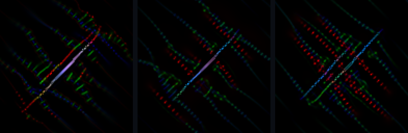
The center panel tests the actual objective: whether the fitted rule maintains the supplied field. The right panel asks a separate question. Starting the same rule from generic noise produces a coherent body, but not the requested anatomy.
The fitted rule maintains the supplied anatomy over the recorded rollout. The full compiler must also discover a compact starting pattern and the rule that develops it into the requested body.
Orbium lets us ask how much a mature body reveals when we already know the kind of rule that made it. We supplied its update law, kernel, growth function, and starting cells, then hid three numerical parameters: the interaction radius R, growth center m, and growth width s. Each candidate develops from those same starting cells and is compared with the reference body at step 600.
We fixed Orbium’s update rule and one-kernel geometry, then searched for the three parameter values. Other update laws and kernel layouts are outside this comparison.
The search starts from R=10, m=0.12, and s=0.024. These values disperse the initial cells into a ring and small fragments.
The first stage evaluates 2,688 parameter combinations. Every candidate runs for 600 steps.
28 × 96 rolloutsThe second stage evaluates 1,152 candidates near the broad-search winner. The selected rule is then run to step 1,200.
12 × 96 rollouts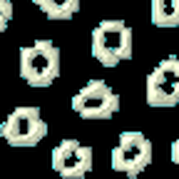
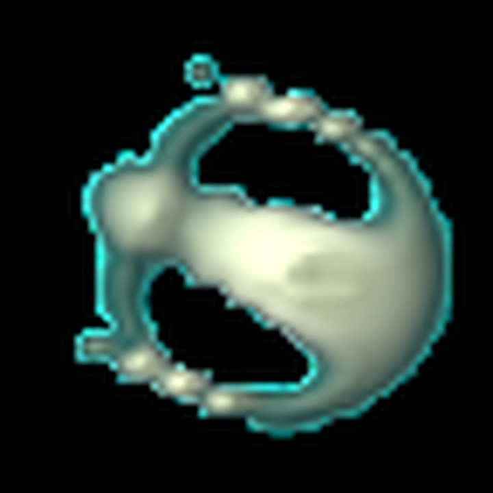
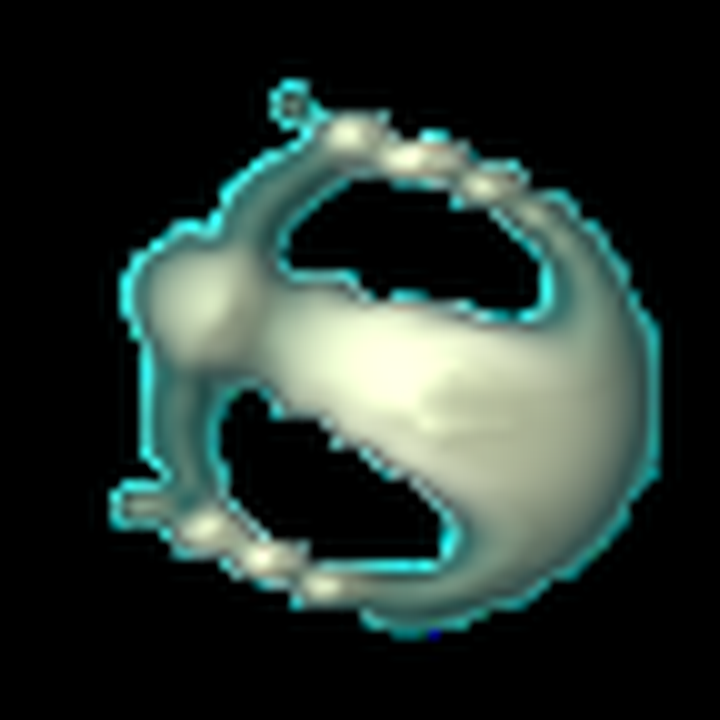
The initial parameters fail. The fitted parameters produce a close reconstruction. Each candidate is simulated for 600 steps, then its complete field is compared with the reference field.
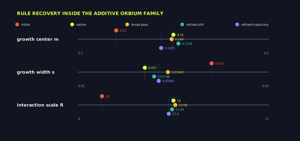
The narrow second stage improved the field match from 0.878 to 0.969 and brought all three hidden values close to the native rule.




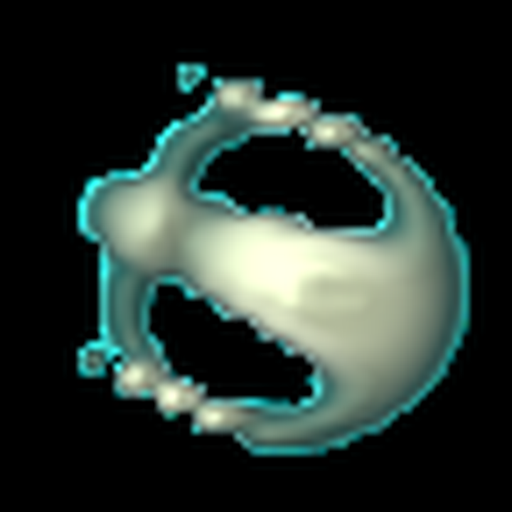

The fitted parameters also produced a coherent body at the unscored steps. This experiment isolates parameter recovery by supplying the update family, kernel geometry, growth function, starting cells, and elapsed time.
A control search used steps 100, 300, and 600. It returned R=12.80, m=0.1435, and s=0.0185. Its replay also remained coherent through step 1,200.
Both runs used the same broad and refinement budgets. The three-frame run ended farther from the hidden values than the run scored only at step 600. This is one organism, so it does not establish that single-frame targets are generally better.
The reconstructions raise a question about the whole collection: how many different rules can fit a similar body? We represent each body by its measured phenotype and call the set of compatible rules a fiber. If that set is broad, choosing a measured form still leaves considerable freedom in the dynamics that produce it.
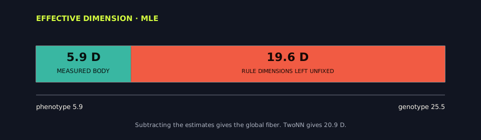
The corpus occupies about 25.5 intrinsic rule dimensions and 5.9 intrinsic phenotype dimensions. Their 19.6-dimension difference (20.9 with an alternative estimator) is estimated from the geometry of the samples; it is not the raw count of 40 parameters minus 15 measurements.
5,000 forms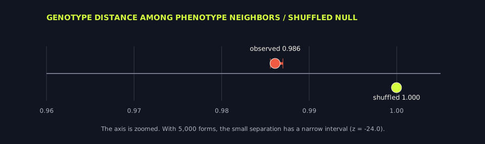
The ratio is 0.986, where 1.0 means that nearby measured bodies are no closer in rule space than shuffled pairs. The difference from 1.0 is detectable, but it is small.
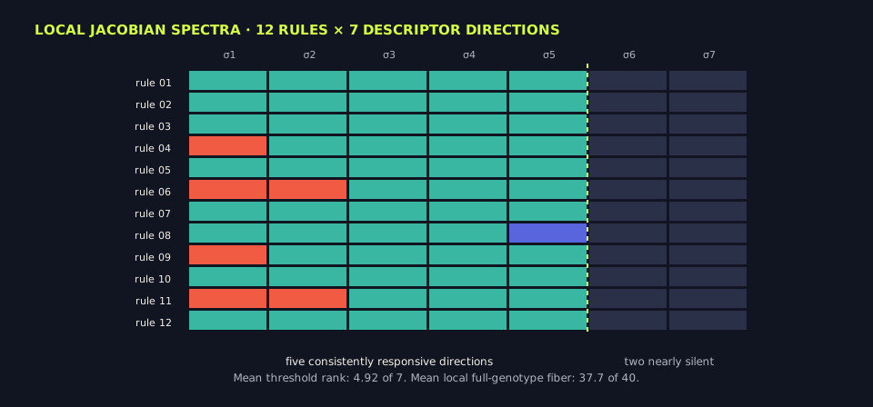
This local test perturbed 12 rules and followed seven descriptors. About five response directions crossed the threshold, but most sensitivity was concentrated in roughly 2.3 effective directions.
12 local probesThe 19.6 and 37.7 dimension estimates answer different questions. The first compares the global intrinsic dimensions of the 5,000-rule corpus and its 15 measured outcomes. The second subtracts the effective rank of a seven-descriptor local response from the full 40-parameter rule. Both indicate substantial ambiguity and should not be compared numerically.
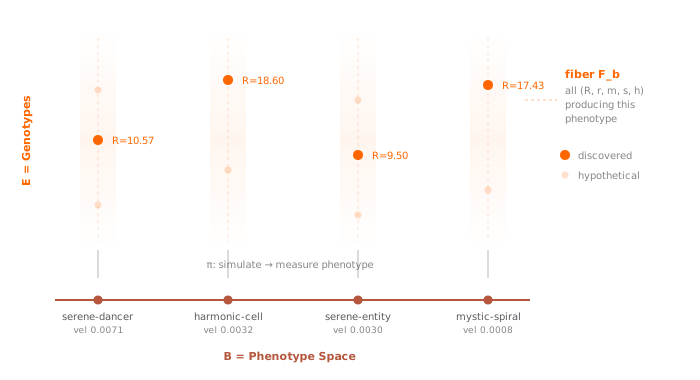
Each point below represents a set of body measurements. The rules compatible with those measurements form the vertical set above it. The geometry is illustrative rather than measured.
schematic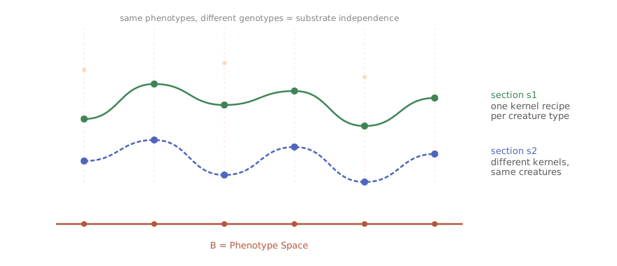
Because several rules can fit the same target, the system needs a policy for choosing among them. Different policies may select rules with different unmeasured dynamics.
schematic
A smooth change in rule parameters can still pass through a region where no viable body develops. Search therefore has to preserve viability as well as reduce distance to the target.
schematicFigures 01A–01C are conceptual diagrams. Figures 02–04 are generated from the frozen anatomical-compiler results.
Retrieving a nearby rule gives the search a starting point; running it reveals whether that proposal produces the requested measurements. Earlier tests examined both parts: whether proposed rules produce stable bodies, and whether simulation-guided refinement improves their match across several targets.
The results below test parts of this system. The conditional proposal check used eight samples across two targets. The refinement result used four targets. The MLX and Swift comparison covered one rule, one starting field, and six steps.
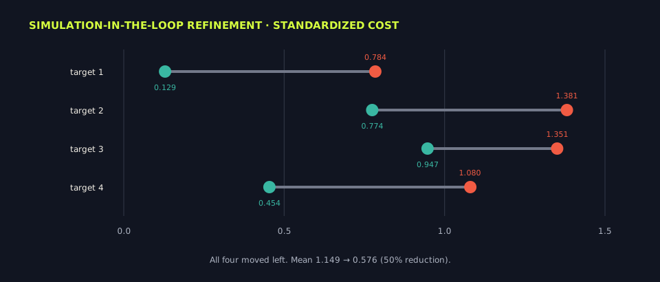
Lower is better on this standardized descriptor distance. Refinement improved all four targets, reducing the mean from 1.149 to 0.576, although one target still ended at 0.947.
four targets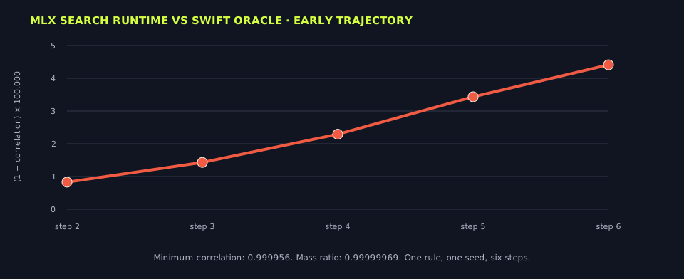
For one genotype and initialization seed, MLX and Swift remained closely aligned through step six. This check covers the beginning of one trajectory.
A body that matches the requested shape may still move differently. To examine that gap, we measured six behaviors in 8,174 creatures and reduced them to principal axes. The first axis is dominated by speed, path length, displacement, and center velocity, so we call it locomotion. The second is dominated by energy and temporal variance, so we call it activity. Together they account for 87.2% of the behavioral variation.
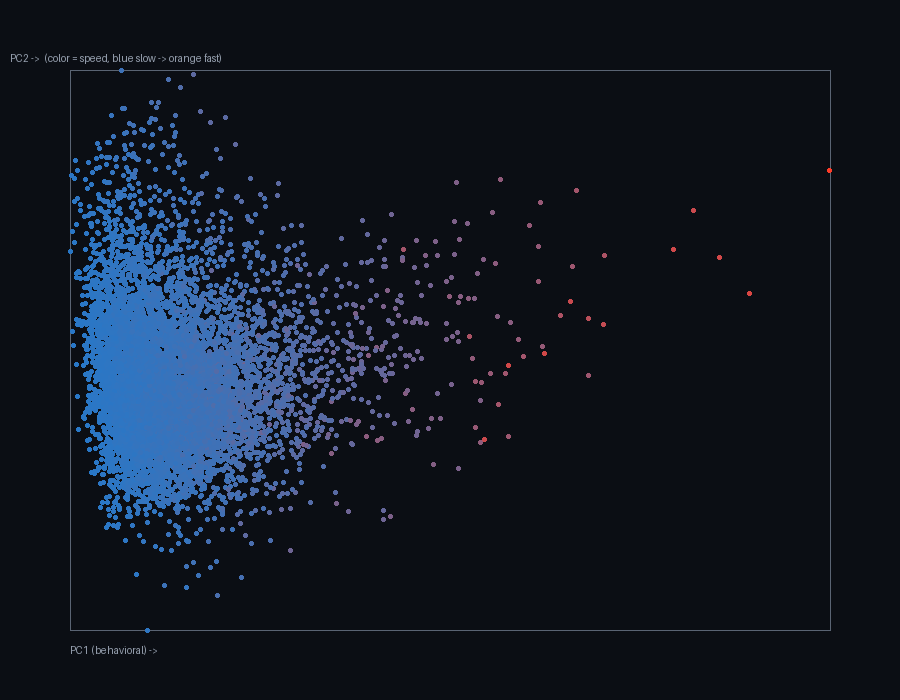
Most creatures occupy a dense low-speed region, while fast locomotion forms a sparse tail. Any model trained on this distribution will see many more slow examples than fast ones.
8,174 creaturesOccupancy and spread helped predict activity. The same shape measurements explained only 3.8% of the locomotion axis. Matching form measurements does not determine how the result will move.
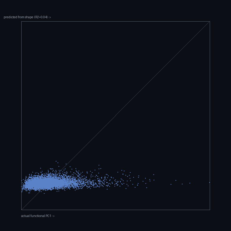
Activity predictions cluster near the diagonal. Locomotion predictions remain compressed near the bottom of the plot.
If many trajectories finish in the same region, it is tempting to picture development as rolling downhill toward it. We tested that picture by fitting a potential surface to the endpoints and comparing its downhill direction with the observed motion. The alignment was weak. In a separate test, five of eight genotypes became more dispersed after their starting conditions were perturbed. Frequent endpoints therefore did not supply the restoring dynamics a compiler would need to rely on.
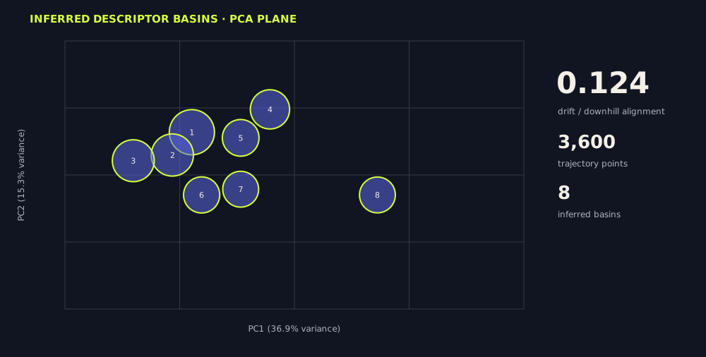
Across 3,600 trajectory points, observed drift aligned with the fitted downhill direction by 0.124. An alignment of 1 would follow the fitted landscape exactly; zero would show no preferred alignment.
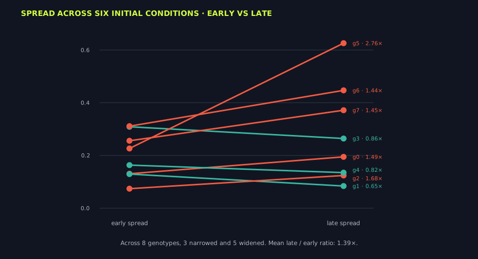
Three rules narrowed the differences between their six initial conditions, while five widened them. The mean late-to-early spread ratio was 1.39, where values above 1 indicate divergence.
8 × 6 rolloutsBulk shape was much more repeatable than motion across starting conditions. Across the same six initial conditions, mean variation was 2.5% for shape and 51% for motion. A rule can produce a broadly consistent form while leaving its trajectory highly contingent on the start.
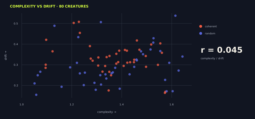
Across 80 creatures, complexity and drift had a correlation of r = 0.045. In this sample, visual complexity provided almost no information about whether a body would remain near its initial location.
80 creaturesThe two searches solve different parts of the problem, maintaining a supplied field and recovering parameters within a known family. None yet discovers both a compact seed and a rule that reliably grows an arbitrary requested body.
The next test should require the search to discover a developmental route: start from a compact seed, grow a withheld target body, and maintain its anatomy. Searching for the seed and rule together would address the part that the supplied-field experiment leaves open. Changed starting conditions and damage would then test whether the fitted dynamics keep producing and sustaining the requested body beyond the trajectory used to select them.
The ledger records the source for every number, specimen, replay, and reused schematic. SHA-256 identifies the exact bytes. The June files do not contain the revision that produced those historical results; the September case-study entries include their exact configs and media.
| Kind | Source | Bytes | SHA-256 prefix |
|---|---|---|---|
| frozen artifact | stage1_fresh_fiber.json | 1,424 | 1fcae1ea8b1613f7… |
| frozen artifact | stage1_jacobian_fiber.json | 4,632 | 9e5e975176e31401… |
| frozen artifact | stage2_cinn.json | 1,244 | d5ecd3b9f31ca5b6… |
| frozen artifact | stage3_refine.json | 551 | be159631b5f0097f… |
| frozen artifact | compiled/demo1/result.json | 1,930 | cf085fb32904ed5f… |
| frozen artifact | compiled/demo1/target.png | 18,649 | de6ebc2862bb8589… |
| frozen artifact | compiled/demo1/creature.png | 16,356 | 53dcf3f8d11f758a… |
| frozen artifact | compiled/demo1_cinn/result.json | 1,889 | a9f5988e1fa3c754… |
| frozen artifact | compiled/demo1_cinn/creature.png | 15,957 | 58e787e1bf2451f2… |
| frozen artifact | compiled/form_demo/result.json | 6,826 | 044567fdf4ea014c… |
| frozen artifact | compiled/form_demo/form_compile.png | 66,658 | b3b03d35b8af0ba2… |
| frozen artifact | mlx_validation.json | 1,039 | 79316f3cb993eef9… |
| frozen artifact | qd_archive/archive.json | 350,936 | 614a1919941427fd… |
| frozen artifact | qd_archive/coverage.png | 2,321 | a6ed57c87e362506… |
| frozen artifact | waddington_flow.json | 2,141 | 6537452489f02b52… |
| frozen artifact | canalization.json | 2,357 | c5a5924d1ae5c946… |
| frozen artifact | functional-morphospace/functional_morphospace.json | 1,685 | e8f6e4b61b319865… |
| frozen artifact | functional-morphospace/shape_function_coupling.json | 1,398 | b9923f08f942351a… |
| frozen artifact | functional-morphospace/functional_morphospace.png | 65,958 | 52f66e8726ea151a… |
| frozen artifact | functional-morphospace/shape_predicts_function.png | 13,462 | 101f3f6ed749b081… |
| frozen artifact | 3c15/functional_map_mlx/functional_map.json | 9,209 | e69a9cec67faaa34… |
| frozen artifact | 3c15/functional_map_mlx/bodies_montage.png | 139,541 | 55b2a1b2466e1bab… |
| reused explanatory schematic | site/assets/blog/lenia-morphospace-report/fig-fiber-bundle.svg | 4,621 | 43000b7e7db2b7c0… |
| reused explanatory schematic | site/assets/blog/lenia-morphospace-report/fig-sections.svg | 4,182 | 569fec81d4c9dd71… |
| reused explanatory schematic | site/assets/blog/lenia-morphospace-report/fig-bridge-genotype-phenotype.svg | 3,035 | 363d5905c657c2e8… |
| 2026-09-02 within-family Orbium inverse | orbium-system-id-v5/experiment.json | 1,284 | e7d17cd2fca63593… |
| 2026-09-02 within-family Orbium inverse | orbium-system-id-v5/still-es.json | 197,817 | c8262451e333bf09… |
| 2026-09-02 within-family Orbium inverse | orbium-system-id-v5/still-run/best.json | 141 | 2e99f52c9591bc8c… |
| 2026-09-02 within-family Orbium inverse | orbium-system-id-v5/still-run/history.jsonl | 12,161 | 540933e403833518… |
| 2026-09-02 within-family Orbium inverse | orbium-system-id-v5/trajectory-es.json | 591,583 | dbb42ebb131bbec6… |
| 2026-09-02 within-family Orbium inverse | orbium-system-id-v5/trajectory-run/best.json | 143 | 97902a5fa38d9c4f… |
| 2026-09-02 within-family Orbium inverse | orbium-system-id-v5/trajectory-run/history.jsonl | 12,205 | b3d53ac97bb5e77a… |
| 2026-09-02 within-family Orbium inverse | orbium-system-id-v5/report-assets/orbium-initial-600.png | 255,120 | 040ffb2271b6a55b… |
| 2026-09-02 within-family Orbium inverse | orbium-system-id-v5/report-assets/orbium-inverse-summary.json | 1,271 | 904916197598ed88… |
| 2026-09-02 within-family Orbium inverse | orbium-system-id-v5/report-assets/orbium-rule-recovery.svg | 6,418 | a0125a9a26e7e89b… |
| 2026-09-02 within-family Orbium inverse | orbium-system-id-v5/report-assets/orbium-still-100.png | 187,493 | 88843f7bf4824041… |
| 2026-09-02 within-family Orbium inverse | orbium-system-id-v5/report-assets/orbium-still-300.png | 186,697 | b7b91bc0d08bd62f… |
| 2026-09-02 within-family Orbium inverse | orbium-system-id-v5/report-assets/orbium-still-600.png | 185,894 | e7eab62cced81915… |
| 2026-09-02 within-family Orbium inverse | orbium-system-id-v5/report-assets/orbium-still-1200.png | 189,664 | 4c4cdf26049b32a0… |
| 2026-09-02 within-family Orbium inverse | orbium-system-id-v5/report-assets/orbium-still-zoom.mp4 | 812,518 | 37933bf5d5c5bb09… |
| 2026-09-02 within-family Orbium inverse | orbium-system-id-v5/report-assets/orbium-target-100.png | 186,009 | 2befab83732f67c4… |
| 2026-09-02 within-family Orbium inverse | orbium-system-id-v5/report-assets/orbium-target-300.png | 187,779 | 2aacf01203662f32… |
| 2026-09-02 within-family Orbium inverse | orbium-system-id-v5/report-assets/orbium-target-600.png | 186,927 | e0ca77a833258f14… |
| 2026-09-02 within-family Orbium inverse | orbium-system-id-v5/report-assets/orbium-target-1200.png | 186,735 | 2d39c4a8ffcb94ed… |
| 2026-09-02 within-family Orbium inverse | orbium-system-id-v5/report-assets/orbium-target-zoom.mp4 | 834,738 | 12c499769fe12ce6… |
| 2026-09-02 narrow Orbium refinement | orbium-system-id-v6-refine/refine-es.json | 197,819 | 7bcda98c84215935… |
| 2026-09-02 narrow Orbium refinement | orbium-system-id-v6-refine/refine-run/best.json | 143 | 43c2f254196e5526… |
| 2026-09-02 narrow Orbium refinement | orbium-system-id-v6-refine/refine-run/history.jsonl | 5,165 | e28679376dddcbf6… |
| 2026-09-02 narrow Orbium refinement | orbium-system-id-v6-refine/trajectory-refine-es.json | 591,585 | 840f48b9aab5b4be… |
| 2026-09-02 narrow Orbium refinement | orbium-system-id-v6-refine/trajectory-refine-run/best.json | 140 | 93cfbf398087a085… |
| 2026-09-02 narrow Orbium refinement | orbium-system-id-v6-refine/trajectory-refine-run/history.jsonl | 5,192 | 7b2bca59b1f57f3b… |
The June and September evidence have different provenance. The frozen June artifact JSON files do not record their source revision, so artifactProducingRevision remains empty. The September within-family Orbium inverse is listed separately with exact configs, results, frames, and videos. The complete machine-readable ledger is source-manifest.json.